


Tom, Tapestry’s Director of Analytics, is a nerd. He likes nothing better than diving deep into a topic and getting lost in its eccentricities. Someone once made the mistake of asking him about research theory and 15 years later he’s still going. We challenged him to condense these ideas into a series of blog posts: He is geeking-out so you don’t have to.
Probably the question we get more than any other is “What is the minimum sample size?”. This is such a common question that it’s often answered on auto-pilot and we don’t explore the reasons behind our recommendations. So, as we’re talking, let’s take the time to look at this most fundamental of questions.
First, let’s talk about sampling.
When we want to know something about a population we have a few options. The best option is to measure every member of the population. In science this is sometimes possible, but in market research it is almost always an impossibly impractical undertaking. Assuming you don’t have a spare £900 million to fund a census, you’re going to need to take a sample instead.
Sampling is simple. You take a small group of the base population and use them to make judgements about the population. There are lots of things we can do to make that sample a better approximation of the population, but the idea is always the same; a small subset is used in lieu of the whole.
Before we move on I’d like pause and talk balls.
The classic example you’ll find in most textbooks is about drawing coloured balls from a bag (or an urn if you’re fancy). You have 20 red balls and 5 blue and you put them in a bag because… well, life is long and you’re bored. In this case, we know the instance of blue balls in the population is 20% – 1 in 5 balls is blue. Now, because it’s raining outside you reach into your bag and fish out a sample of 5 random spheres.
That is what you’re doing every time you take a sample; playing with your balls. Childish jokes aside, it’s a helpful example. But hang on, you’re thinking, the probability of a single draw being blue might be 20%, but there’s no guarantee the 5 balls we draw will match the 1 in 5 distribution we know to be true. We’re not going to go into the probability of that draw, but you’re right: your sample will be a mixture of red and blue balls, or you may have no blues at all. And if you put everything back and did it again, you might well get a different result.
The point is, samples aren’t populations: they can be off in their estimates. How off they are depends on a few factors and perhaps the easiest to change (though not always the cheapest) is the sample’s size. The larger the sample, the better the chance of getting at that population incidence.
Now, finally, we get to the meat of the sandwich.
Imagine we have a new bag of balls, this time there are 1000 black and white balls and their distribution is unknown – we don’t know how many of each there are. This is more similar to the problem we face in market research: I have 1000 consumers and want to know how many will buy a product.
If I take out 10 balls from this new bag, I’ll have an incidence of black/white. Instinct tells you to be cautious of that incidence with just 10. It’s too small a sample. But why?
The answer is known as the ‘margin of error’. This is effectively the degree of confidence we have in our sample’s distribution representing the population’s distribution. If we repeated our draw of 10 black/white balls, we’d expect the result to be different to the original draw but, as we repeated these draws, we’d find a pattern emerging. The incidences would form a normal distribution (a bell-curve) around the true incidence in the bag.
If we drew bigger samples (say, 100), we’d get a narrower distribution as the incidences are more similar. And that is the point: larger samples provide a narrower margin of error so we can be more confident about our sample representing the population.
To get specific, the fact that this distribution is ‘normal’ is very useful because the normal distribution has some known properties. For instance, we know that 68% of draws will be one standard deviation or less away from the true score and 95% will be 2 away (well, 1.96). As 95% of samples are in that margin, the likelihood is that your sample estimate is too. This is also known as a confidence interval*: the bounds we are confident future samples will fall into and our ‘true’ value will reside.
Therefore, knowing what the sample’s own margin of error is gives us an approximation of the population’s margin and the true value of our measure**. We’re not going to go into the algebra of how to calculate the margin of error, but the concept should be clear to you now: it is the limits of what we’re prepared to say the ‘true’ score in the population is.
Remember, the larger the sample, the narrower the margin of error. With a sample of 10, the margin of error is quite wide – around ±30% – so we can only say that 95% of the samples and, in all probability, our true value, we take are within a 60% window (our estimate plus or minus 30%). If we were to take a sample of 100, the margin shrinks to ±10%. With 1000 it’s ±3% (although our bag is now empty and we have measured the whole population). This image makes it nice and clear what’s happening:
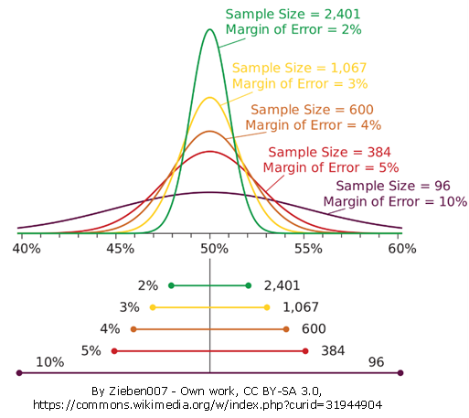
The conclusion, then, is clear. More sample means a narrower margin of error and more confidence about our data reflecting the ‘true’ score of the population. So, when someone asks you “What is the smallest sample size we can use?” you know that the answer depends on how vague they’re willing to be: fewer than 100 people and your conclusions will be wobbly as you can only claim your answer is within a 20% interval.
Now you just need to find someone to pay for some extra sample.
*While these are similar, they’re not quite the same. A margin of error is presented often as a single number, described as ‘plus or minus’ (as represented by this symbol: ±). For example, human short-term memory holds 7 items, with a margin of error of plus or minus 2 (can range from 2 more than 7 to 2 less than 7). Meanwhile a confidence interval is expressed as a range (from 5 to 9, centred on 7)
**There are some common interpretation mistakes which even experienced scientists make on this, but they make understanding the concepts more difficult so should only be explored when you’re comfortable*** with the ideas presented here.
***Comfortable? Great. The common interpretation of a margin of error or a confidence interval is that there is a 95% chance of the true value being within those margins. However, this is not actually what it does. A confidence interval is a mathematical or probabilistic object. That is, it only exists in probability – there is a 95% chance that the (95%) confidence interval of a future sample will cover the true value. As soon as a confidence interval is observed, it collapses and either does or does not include the true figure. The point is that 95% of those collapsed intervals will include the true variable not that your calculated interval does.